How to install the Lucidchart add-in for Excel
First, download the Lucidchart add-in for Excel. To do so, follow these simple steps:
- Open Excel.
- Go to Insert > Add-in > Get add-in.
- Search and select “Lucidchart Diagrams for Excel.”
- Click “Add.”
- Accept the terms and conditions.
- Log in with your Lucidchart credentials to access your documents.
Install the add-in
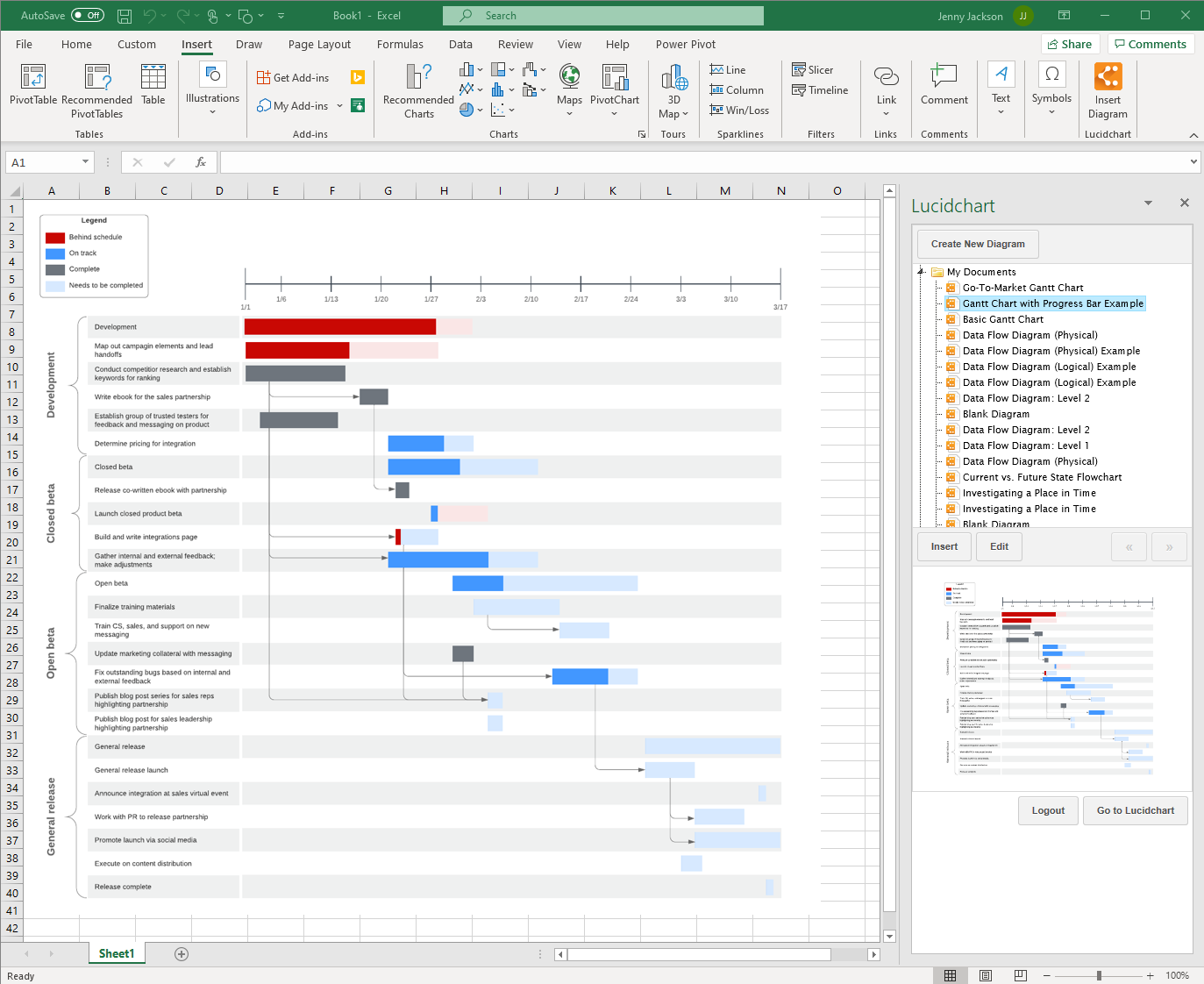
How to insert a Gantt chart into Excel with the Lucidchart add-in
Insert a Gantt chart into your spreadsheet, as a high-resolution image, without ever leaving Excel.
- In Excel, find the Lucidchart button in the upper-right corner.
- Click ”Insert Diagram.”
- Select your Gantt chart from the list.
- A preview will appear in the bottom box. If it is the correct document, click “Insert.”
- To edit your Gantt chart, select “Edit.” Make the necessary changes in the pop-up window and then click “Insert” to update your diagram.
How to build a Gantt Chart in Excel with the Lucidchart add-in
Create and edit your own Gantt chart in Excel using the Lucidchart editor within the Microsoft add-in.
- In Excel, select “Insert Diagram” to open the Lucidchart panel.
- Click “Create New Diagram.”
- Choose either a blank document or template to start.
- Drag and drop shapes and edit the text to build your Gantt chart.
- Save your Gantt chart and click back into your Excel spreadsheet.
- Select your new diagram from the sidebar and click “Insert.”

Visit our Help Center or watch the video tutorial below for additional instructions on installing and using the Lucidchart add-in.
Option #2: Manually make a Gantt chart in Excel
You can still make a Gantt chart from scratch in Excel following the steps listed below. But keep in mind that the process will be more time-consuming and less intuitive than using Lucidchart and you won’t have the opportunity to use pre-made templates.
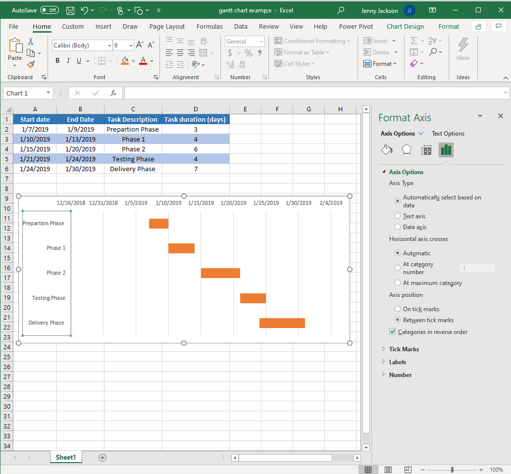
Format your data and select your bar graph
- Input and title each column: “Start Date,” “End Date,” “Task Description,” and “Task Duration.”
- Add your project data to the spreadsheet.
- Go to Insert > Chart > Bar chart > Stacked bar chart.

Add data to your Gantt chart
- Right-click on the chart and find “Select data.” A “Select Data Source” box will appear.
- Click “Add.” An “Edit Series” dialog box will appear.
- Select the “Series name” box.
- With your cursor in the “Series Name” box, select the “Start Date” cell in your worksheet. Click back into the “Series name” box.
- Select the “Series value” box.
- With your cursor in the “Series value” box, select all the values in the “Start Date” column on your spreadsheet. Click back into the “Series value” box. Click “OK.”
- Back in the “Select Data Source” box, click “Add.”
- Repeat the same process for “Task Duration.”


Format your Gantt chart
- Select “Start date” on the left side of the “Select Data Source” box. Then, click the “Edit” button in “Horizontal (Category) Axis Labels.”
- Select the “Axis label range” box.
- With your cursor in the “Axis label range” box, select the values under the “Task Description” in your spreadsheet. Click “OK."
- Select the left-most bars of the horizontal bar graph. Right-click and select “Format Data Series.” A sidebar will appear.
- Select the paint bucket icon. Under the “Fill” options, select “No Fill.”
- Do not close the formatting window. Select the task descriptions on the left of the chart and click on the bar chart icon.
- Under the “Axis options,” click the “Categories in reverse order” checkbox.
Done! You've created your own Gantt chart in Excel.


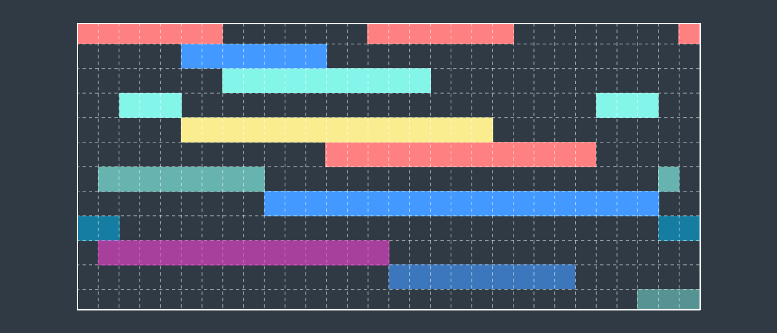
Gantt chart examples
Ensure your project goes off without a hitch when you get started with one of our Gantt chart templates. Just click the template to open it with your Lucidchart account and start editing.